Four-Bar Linkages
A planar four-bar linkage consists of four rigid rods in the plane connected by pin joints. We call the rods:
- Ground link $g$: fixed to anchor pivots $A$ and $B$.
- Input link $a$: driven by input angle $\alpha$.
- Output link $b$: gives output angle $\beta$.
- Floating link $f$: connects the two moving pins $C$ and $D$.
We often think of a four-bar linkage as being driven at the input angle $\alpha$, resulting in the output angle $\beta$. We only need one input, because the system has exactly $N_{\rm DOF} = 1$ degree of freedom. We can count the DOF as 9 free variables (three moving rigid bodies with three variables each) minus 8 constraints (four pin joints with two constraints each).
|
Four-bar linkages can be used for many mechanical purposes, including to:
- convert rotational motion to reciprocating motion (e.g., pumpjack examples below)
- convert reciprocating motion to rotational motion (e.g., bicycle examples below)
- constrain motion (e.g., knee joint and suspension examples below)
- magnify force (e.g., parrotfish jaw examples below)
Rotating cranks and reciprocating rockers
Four-bar linkages can convert between different types of motion. We call these:
- Crank rod: rotating motion through a complete circle.
- Rocker rod: reciprocating motion with a total angle less than $360^\circ$.
On the linkage below, adjusting the lengths of the input rod $a$ and the output rod $b$ shows that we can have an input crank and output rocker or the other way around, depending on whether $a < b$ or $a > b$. The case when $a = b$ is special.
|
| Input link length: | \(a = \) cm | |
| Output link length: | \(b = \) cm |
Coupler dynamics
The joints $C$ and $D$ always move in circles or semi-circles. More complex motion can be achieved with a coupler point $P$ attached to the floating link $f$, as shown below where the position of $P$ can be adjusted. Adding a coupler technically makes this a six-bar linkage (four original links plus $CP$ and $DP$).
Here the input and output links are listed as a 0-rocker and π-rocker, as they reciprocate about the angles $\alpha = 0^\circ$ and $\beta = 180^\circ = \pi\rm\ rad$, respectively.
|
| Coupler position: | \(P_{\rm pos} = \) % from DC midpoint towards C | |
| Coupler offset: | \(P_{\rm off} = \) % of DC length |
Limiting the input angle
It is often helpful to limit the input angle in a mechanism, even when the linkage could allow for greater movement. For example, to have a lifting platform the linkage below uses a crank limited to a smaller reciprocating input range. The input center angle $\alpha_{\rm cent}$ and range $\Delta\alpha$ can be adjusted to control the range of movement of the platform.
|
| Input angle center: | \(\alpha_{\rm cent} = \) % from 0° to 360° | |
| Input angle range: | \(\Delta\alpha = \) % of 180° |
Example: Pumpjack (rotary to reciprocal)
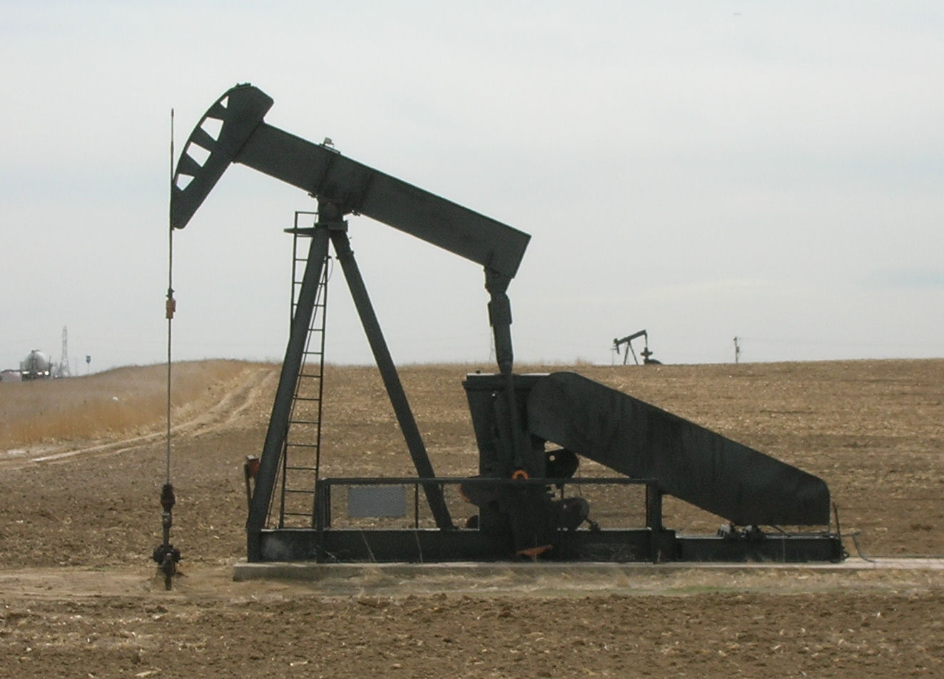
In areas where underground oil is not under enough pressure to drive it all the way to the surface, it is necessary for oil wells to actively pump up the oil. One standard method for achieving this is to use a reciprocating piston that pumps the oil up the shaft. As most motors (electrical or internal combustion) provide a rotating drive shaft, some way is needed to convert the rotary engine motion into reciprocating pump motion. A pumpjack is a drive mechanism to achieve this, consisting of a four-bar linkage as shown below. The heavy rotating counterweight is arranged so that it is falling while the pump is performing the up-stroke, and thus lifting the oil against gravity. This allows a smaller engine to be used.
A pumpjack (also known as a nodding donkey) pump in Northeast Colorado. Image credit: Flickr image by Greg Goebel (CC BY-SA 2.0) (full-sized image).
Example: Bicycle pedaling (reciprocal to rotary)
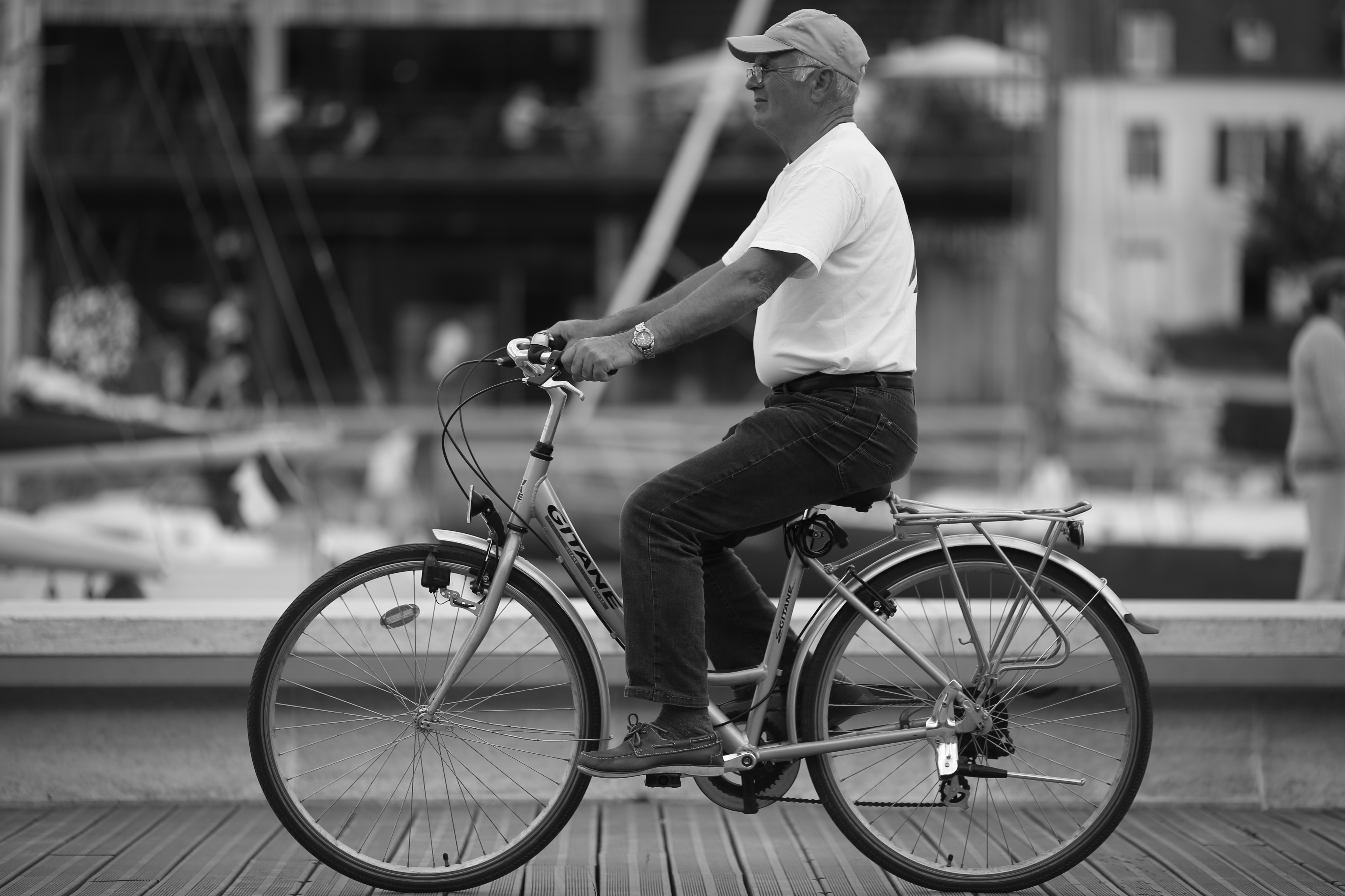
Bicycles are an efficient means of human-powered transportation due to their use of rotary wheel motion. Humans cannot directly produce indefinite rotations, however, so some mechanism is required to translate reciprocating human motion into rotary motion. Bicycles achieve this conversion with two four-bar linkages, each consisting of the two segments of the riders leg, the bicycle frame, and the crank, as shown below.
A man riding a bicycle at the port of Vannes, Brittany, in the north-west of France. Image source: Flickr image by Alexandre Dulaunoy (CC BY 2.0) (full-sized image).
While the four links in the bicycle linkage are approximately rigid rods, only two of the joints are in fact reasonable models of a pin joint (the knee and lower crank). At the pedal and seat, only compression is allowed, as there is no way for the rider to pull up on the pedal or seat. This doesn't normally matter, as the rider's weight serves to maintain the connection at the seat, while the pedal joint only has force exerted during the down-stroke on each side, and the two legs are offset by 180° so one is always pushing down. An alternative approach is used on racing bikes, where the feet are clipped to the pedals and so each foot can pull up as well as push down.
While the current form of the bicycle may seem obvious, with a rotary crank connected by a chain to the rear wheel, it took over 50 years for it to be developed. Before this time, many different systems for bicycle propulsion were tried. The first bicycle, invented by Karl Drais in Mannheim, Germany in 1818, used direct human propulsion along the ground, as shown below. Mannheim was an important location for vehicle invention, as it was also the city where Karl Benz invented the modern automobile in 1885.
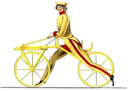
Image credit: Wikimedia Commons (public domain) (full-sized image).
Later bicycle propulsion mechanisms used pedals directly attached to the hub of the front wheel (the so-called bone-shaker), which caused difficulties in pedaling while turning. This direct drive also had gearing problems, as a comfortable ratio of pedal frequency to velocity required very large wheels, leading to the penny-farthing. An alternative approach to cranks was to use treadles, allowing the pedals to be positioned away from the wheel hub. This series of inventions finally resulted in the safety bicycle in 1876, which is the modern form we still use today.
Example: Knee joint (constrained motion)
The human knee joint is a type of biological hinge, which allows movement in only one primary angle. The knee connects the femur (the upper leg bone) to the tibia (the larger of the two lower leg bones). These two bones sit next to each other and are free to rotate about a single axis. A mechanism is needed to keep the two legs bones attached to each other, while still allowing rotation. In the case of the human knee this is achieved with a four-bar linkage consisting of the two bones together with the anterior cruciate ligament (ACL) and posterior cruciate ligament (PCL), as shown below.
An MRI image of a sagittal section through a human knee joint, showing the ACL and PCL ligaments. Image credit: Wikimedia Commons image (CC BY-SA 2.0).
The four-bar model of the knee is only approximate, and neglects many important mechanical features. In particular, the ACL and PCL are not rigid rods, and can only provide tensile forces (they act as mechanical ropes). The compressive force is actually provided by the meniscus that separates the femur and tibia bones. In the simple four-bar knee model shown here, the rigid rods include the effects of both the ligaments and the meniscus.
References
- A. B. Zavatsky and J. J. O'Connor. A model of human knee ligaments in the sagittal plane: Part 1: Response to passive flexion. Proceedings of the Institution of Mechanical Engineers, Part H: Journal of Engineering in Medicine, 206(3):125–134, 1992. DOI: 10.1243/PIME_PROC_1992_206_280_02
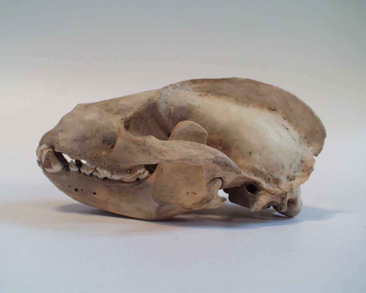
No joints in the human body have the rotating bone fully constrained by the enclosing socket bone. Instead, like the knee, they have a partial socket or cylinder and the rotating bone is held in place by ligaments. This type of arrangement is typical for most animals, with one rare exception being the European Badger (Meles Meles). In older badgers, the jaw rotates on an entirely enclosed pivot, as shown below. This means that the badger cannot waggle its jaw side-to-side as humans can, and also means that the badger jaw cannot be dislocated or disconnected without breaking the bone.
Image credit: Wikimedia Commons (CC BY-SA 3.0) (full-sized image).
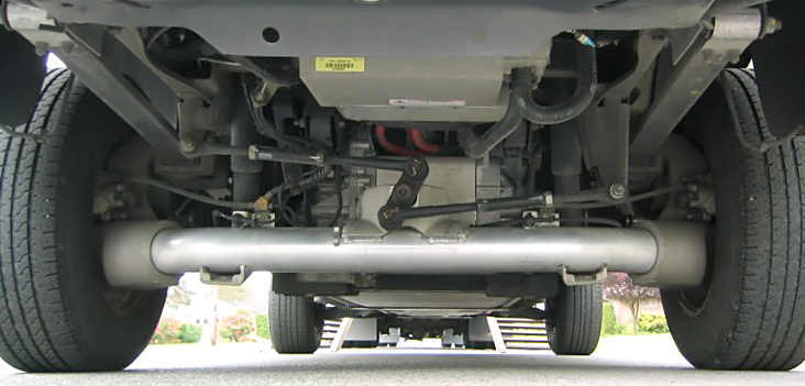
Example: Suspensions with Watt's linkage (constrained motion)
Apart from being one of the inventors of the steam engine and having an SI unit named after him, James Watt also developed a linkage to produce approximate straight line motion. Watt's linkage consists of two long near-parallel links and a small floating link between them, with the near-linear motion occurring for a coupler point midway along the floating link. This linkage is commonly used in suspension systems, as shown below.
The rear suspension of a 1998 Ford Ranger EV. Image credit: Wikimedia Commons (CC SA 1.0) (full-sized image).
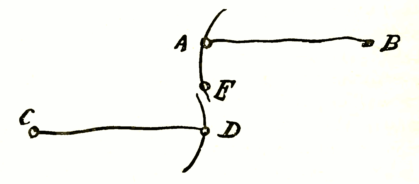
Watt's original hand drawing of the linkage clearly shows the main elements, and also indicates the circular motions of the two moving pivots, as we can see below.
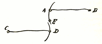
Watt's hand-drawn diagram explaining the concept behind his new linkage design. Image credit: Wikimedia Commons, originally from J. P. Muirhead, The Life of James Watt with Selections from his Correspondence, 1858, p. 294 (public domain) (full-sized image).
The discovery was first revealed in a letter that Watt wrote in 1784:
I have got a glimpse of a method of causing a piston rod to move up and down perpendicularly by only fixing it to a piece of iron upon the beam, without chains or perpendicular guides [...] and one of the most ingenious simple pieces of mechanics I have invented.
While Watt's linkage only produces approximate straight-line motion, the 8-link Peaucellier-Lipkin linkage, shown below, was discovered in 1864 and produces an exactly straight line. In the illustration the links of the same color are equal in length.
Rather than trying to discover special linkages to produce different types of motion, Alfred Kempe proved that any plane algebraic curve (the set of zeros of a polynomial like \(x + 2 x^3 - y^2 - 3\)) can be traced by a sufficiently complicated linkage. See: A. B. Kempe, On a General Method of describing Plane Curves of the nth degree by Linkwork, Proceedings of the London Mathematical Society (1875) s1-7(1): 213-216. doi: 10.1112/plms/s1-7.1.213.
Example: Parrotfish jaw (force multiplication)
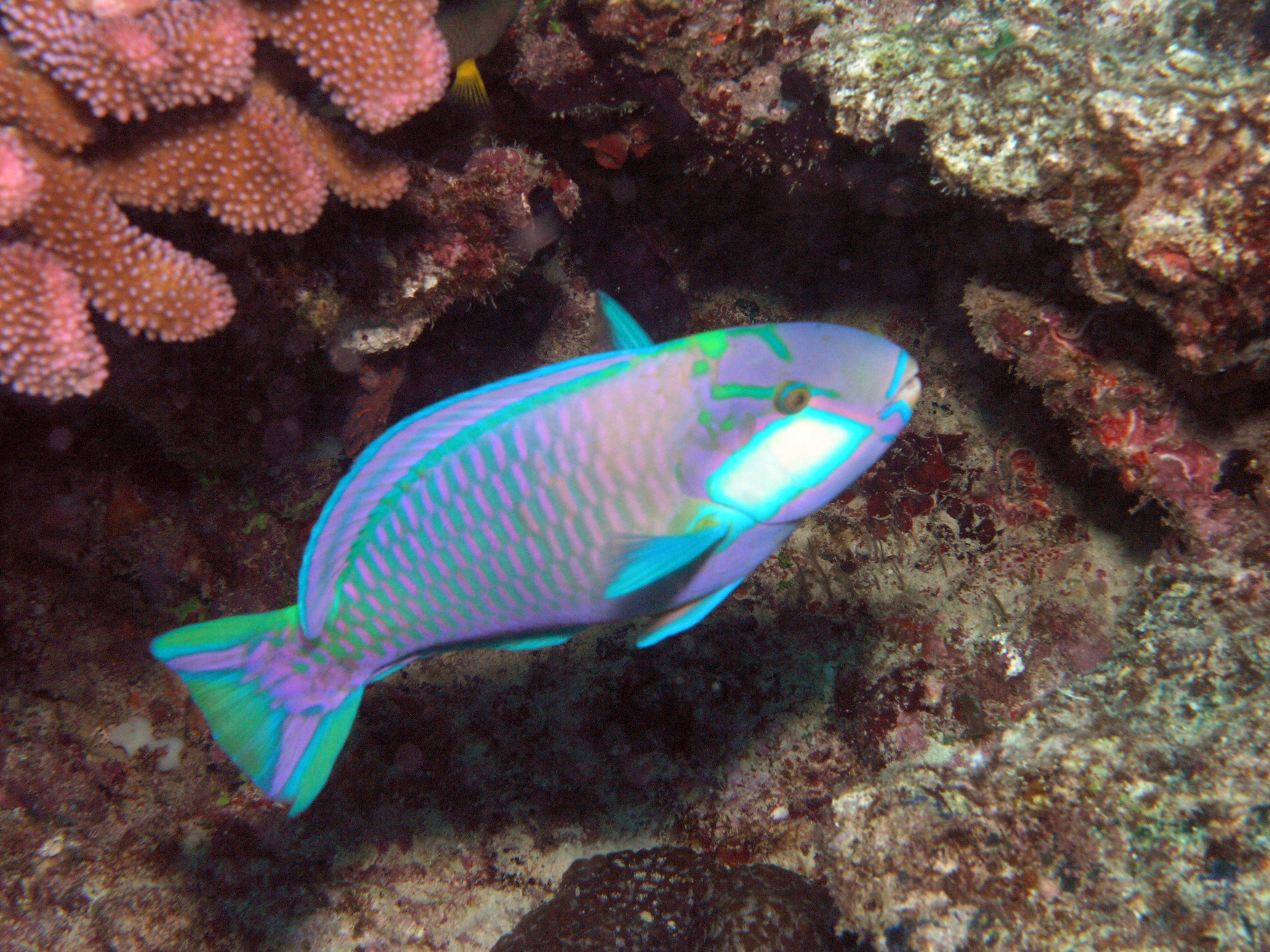
Parrotfish live in shallow tropical waters on coral reefs, where they feed on the the algae that live inside the coral. To get to the algae, they eat the coral itself and then grind it up to release the algae-filled coral polyps inside. The name of parrotfish comes from their teeth, which are packed tightly together to form a parrot-like beak and which grow continuously as they are worn down by feeding.

A Bleeker's Parrotfish (Chlorurus bleekeri) swimming in front of coral in Fiji. Image credit: Image reef4416 from NOAA's Coral Kingdom Collection by Julie Bedford. (Public domain, U.S. Federal Government). (full-sized image).
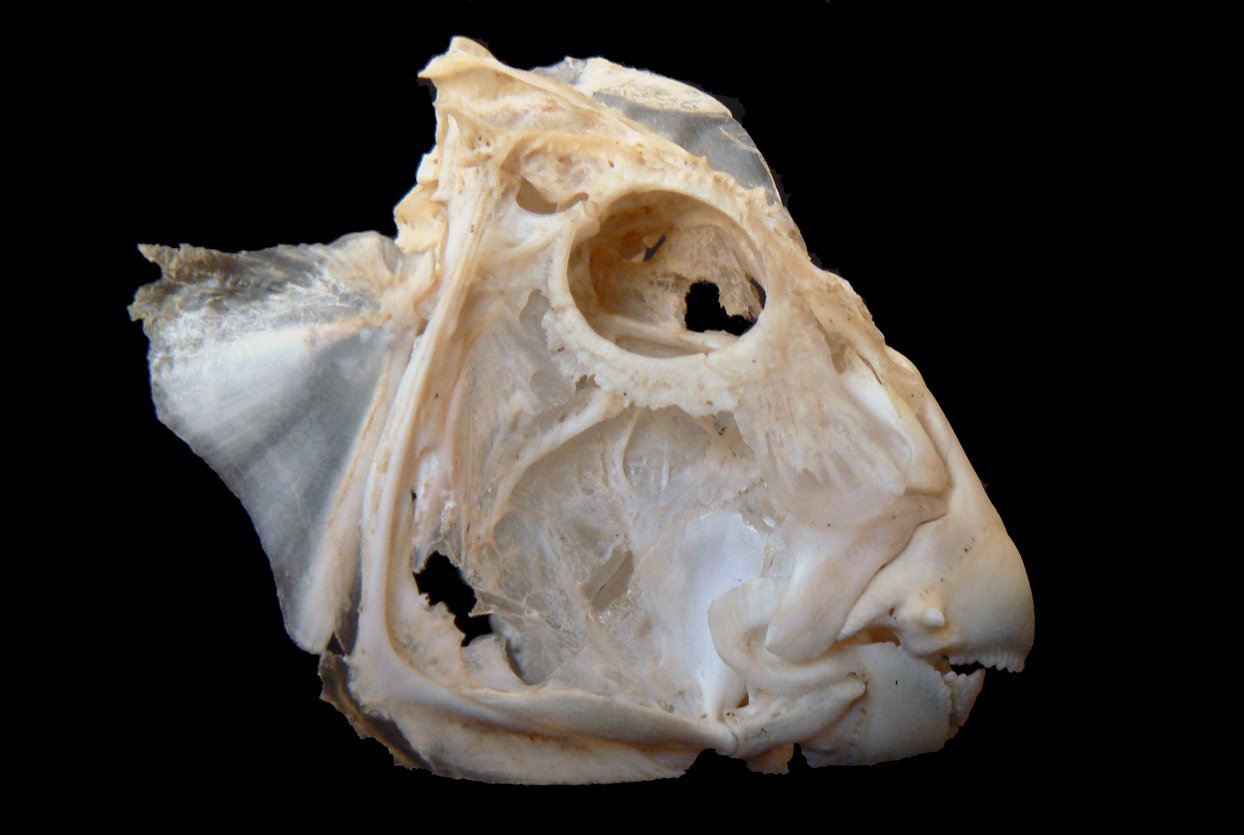
To eat the calcium carbonate coral skeleton, parrotfish need not only extremely strong teeth, but they also need a very powerful biting motion of their jaws. To achieve this, they use a four-bar linkage in their jaws to enable the muscle force to obtain a significant mechanical advantage when the jaws are closing, as shown below. The opening motion is comparatively weak, but this is unimportant for normal feeding.
The skull of a Bleeker's Parrotfish, showing the main components of the jaw. Image credit: BioLab image by Pavel Zuber (CC BY 2.0) (full-sized image).
References
- M. Muller. A Novel Classification of Planar Four-Bar Linkages and its Application to the Mechanical Analysis of Animal Systems. Philosophical Transactions of the Royal Society B, 351(1340):689–720, 1996. DOI: 10.1098/rstb.1996.0065
Parrotfish have two sets of jaws: the regular set of oral jaws that we can see, and a second set of pharyngeal jaws located at the start of their throat (the pharynx). The pharyngeal jaws are used to crush the coral that has been bitten off by the main oral jaws.
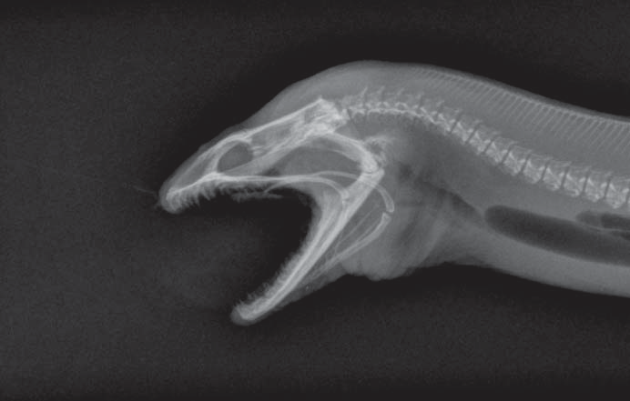
Many species of fish have secondary pharyngeal jaws. A particularly striking example is the Moray eel, shown below, which launches its pharyngeal jaws up into the mouth to actively capture prey and drag it back into the throat. This is the basis for the Alien from the film series, which could launch its inner pharyngeal jaws well beyond its body.
Image credit: R. S. Mehta and P. C. Wainwright, Raptorial jaws in the throat help moray eels swallow large prey, Nature 449, 79-82, 2007. DOI: 10.1038/nature06062. (full-sized images: closed, open).
Full linkage model
The linkage model below can have its geometry set either by the link lengths ($g$, $a$, $b$, $f$) or by the excess quantities ($T_1$, $T_2$, $T_3$). Whether each of the $T_i$ are positive or negative determines the type of input and output (crank, rocker, etc.). For example, if $T_3$ is negative then $T_3 = f + b - g - a < 0$, which means $g + a > f + b$. This implies that the input angle $\alpha$ cannot rotate around to $180^\circ$, as $D$ would be too far from $B$, and so the input rod can't be a crank and must be some type of rocker.
Two other useful geometric quantities shown below are the Grashof index $G$ and the validity index $V$. If $G \gt 0$ then the shortest link is able to fully rotate through $360^\circ$ (the linkage is “Grashof”), while if $G \lt 0$ then the shortest link only reciprocates (the linkage is “non-Grashof”). If $V \lt 0$ then the linkage is impossible, as the longest link is longer than the total length of the other three links.
|
| Orientation: | ||
| set link lengths | ||
| Ground link length: | \(g = \) cm | |
| Input link length: | \(a = \) cm | |
| Output link length: | \(b = \) cm | |
| Floating link length: | \(f = \) cm | |
| set excess values | ||
| Ground-free excess: | \(T_1 = g + f - b - a = \) cm | |
| Output-ground excess: | \(T_2 = b + g - f - a = \) cm | |
| Free-output excess: | \(T_3 = f + b - g - a = \) cm | |
| Total length: | \(L = g + f + b + a = \) cm | |
| Coupler position: | \(P_{\rm pos} = \) % from DC midpoint towards C | |
| Coupler offset: | \(P_{\rm off} = \) % of DC length | |
| Ground link angle: | \(\theta_{\rm g} = \) ° | |
| Input angle center: | \(\alpha_{\rm cent} = \) % from \(\alpha_{\rm min}\) to \(\alpha_{\rm max}\) from 0° to 360° | |
| Input angle range: | \(\Delta\alpha = \) % from \(\alpha_{\rm cent}\) to nearest \(\alpha_{\rm min}/\alpha_{\rm max}\) of 180° | |
| Grashof index: | \(G = s + l - p - q = \) cm | |
| Validity index: | \(V = l - s - p - q = \) cm | |
The variables \(s\) and \(l\) are the shortest and longest side lengths, respectively, while \(p\) and \(q\) are the remaining two side lengths.
The type of input and output links is determined by whether each of $T_1$, $T_2$, and $T_3$ are positive, zero, or negative. The full table of possibilities is given below.
| \(T_1\) | \(T_2\) | \(T_3\) | Input \(\alpha\) | Output \(\beta\) | \(T_1\) | \(T_2\) | \(T_3\) | Input \(\alpha\) | Output \(\beta\) | \(T_1\) | \(T_2\) | \(T_3\) | Input \(\alpha\) | Output \(\beta\) |
|---|---|---|---|---|---|---|---|---|---|---|---|---|---|---|
| + | + | + | crank | rocker | + | + | 0 | crank | π-rocker | + | + | - | 0-rocker | π-rocker |
| 0 | + | + | crank | π-rocker | 0 | + | 0 | crank | π-rocker | 0 | + | - | 0-rocker | π-rocker |
| - | + | + | π-rocker | π-rocker | - | + | 0 | π-rocker | π-rocker | - | + | - | rocker | rocker |
| + | 0 | + | crank | 0-rocker | + | 0 | 0 | crank | crank | + | 0 | - | 0-rocker | crank |
| 0 | 0 | + | crank | crank | 0 | 0 | 0 | crank | crank | 0 | 0 | - | 0-rocker | crank |
| - | 0 | + | crank | crank | - | 0 | 0 | crank | crank | - | 0 | - | 0-rocker | 0-rocker |
| + | - | + | π-rocker | 0-rocker | + | - | 0 | π-rocker | crank | + | - | - | rocker | crank |
| 0 | - | + | crank | crank | 0 | - | 0 | crank | crank | 0 | - | - | 0-rocker | crank |
| - | - | + | crank | crank | - | - | 0 | crank | crank | - | - | - | 0-rocker | 0-rocker |