Track transition curves
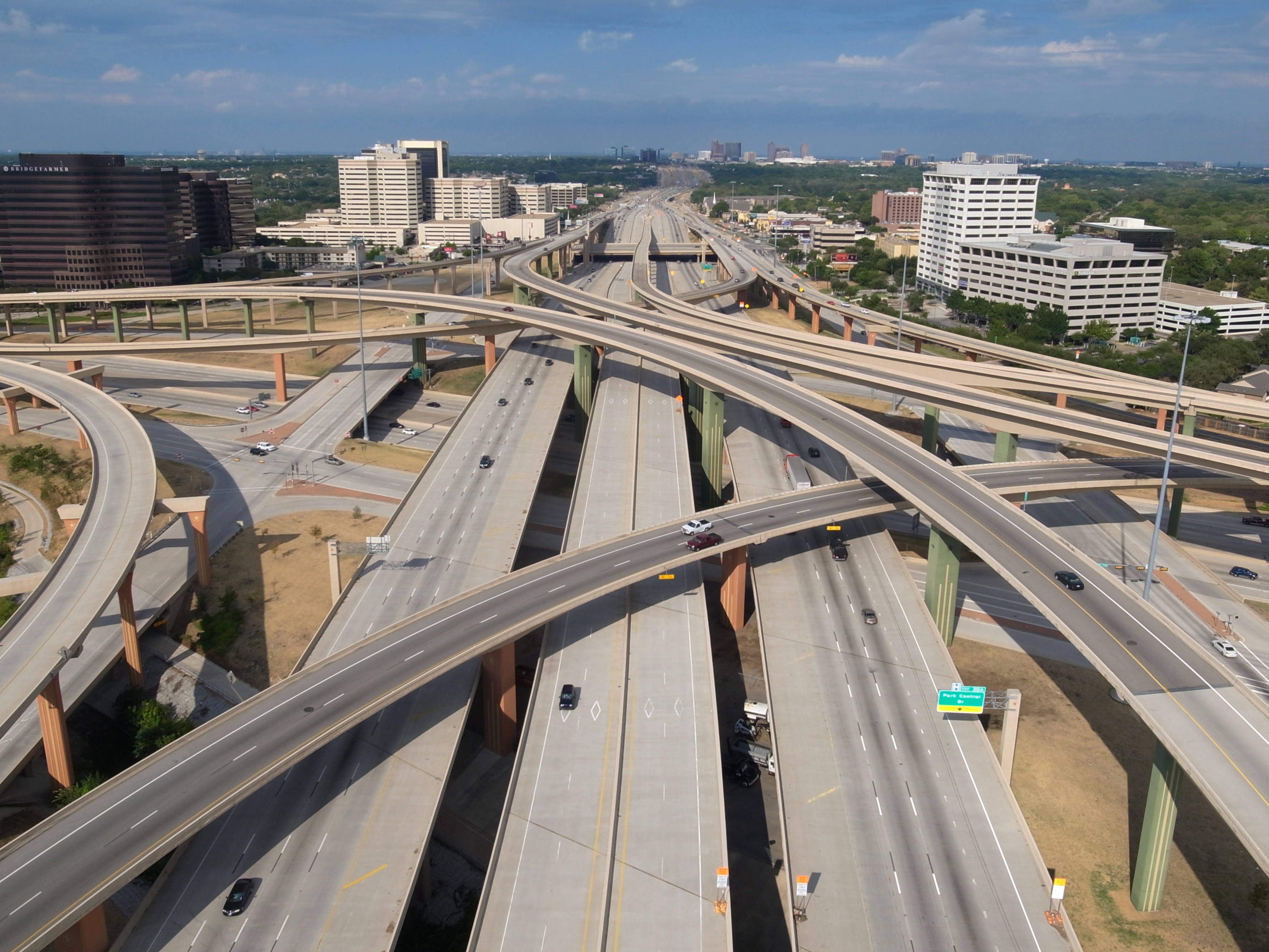
For passengers in a car or train, traveling in a straight line at constant speed is the most comfortable motion, as there is no acceleration. Roads or rail lines with only straight lines are rather limiting, however, so we frequently encounter curves, in the most extreme form in large freeway interchanges such as shown below.
When designing a freeway interchange, one of the most basic questions just what shape the transition curves between the straight-line roads should have. Other considerations then follow, such as stacking the roads above each other and banking the angle of the roads.
The difficultly in designing curves in roads arises from the need to have a smooth ride for the passengers in the vehicles as they traverse the curves at high speed. In particular, we do not want to have sudden changes in acceleration for the passengers.
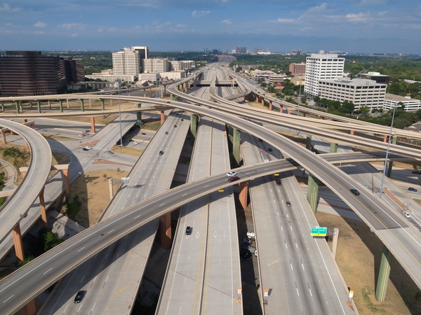
Aerial view of the High Five multi-level stack interchange between I-635 and US 75 in Dallas, Texas, taken with a camera suspended from a kite line. Image source: Fotopedia image, from the flikr image by Jett Attaway (CC BY 2.0) (full-sized image).
Circular arcs for transition curves
To understand the issues with transition curve design, we will consider a simple oval track with two straight segments joined by curves at both ends. The simplest curve shapes are semi-circles (half-circles), as shown below.
Car driving at constant speed around a track with straight line segments joined to perfect semi-circle ends. The graph at the bottom shows the acceleration magnitude versus time. Note the sudden jump in acceleration magnitude when the car switches from a straight line to the curve.
If we the car driving around the track with semi-circle ends, then we see that there is zero acceleration on the straight segments, but on the semi-circular transition curves the acceleration is inwards with magnitude $v^2 / \rho$, where $\rho$ is the radius of curvature. A passenger would thus feel no acceleration on the straight segments, but then would suddenly feel a large sideways acceleration as the vehicle switches to the semi-circles, which would be very uncomfortable and potentially dangerous.
For passenger comfort, we do not want rapid changes in acceleration for transition curves. That is, we want a low value for the derivative of acceleration with respect to time. The derivative of acceleration is known as jerk, defined by $\vec{\jmath} = \dot{\vec{a}}$ (for vectors) or $j = \dot{a}$ (for scalars). With perfect semi-circular ends we see that the jerk is mathematically infinite at the transition to the curve, although in reality it would just be a very high value as the vehicle would not transition to the semi-circle instantaneously.
While the terms velocity and acceleration are standard for the 1st and 2nd derivatives of position, the names for higher derivatives are not so well-established. While jerk is often used for the derivative of acceleration (so the 3rd derivative of position), the terms jolt, surge, and lurch are also sometimes encountered for this quantity. The derivative of jerk is sometimes called jounce (so it is the 4th derivative of position). Another suggestion is to refer to the 4th, 5th, and 6th derivatives of position as snap, crackle, and pop, respectively.
Jerk and snap have many applications in engineering and science. For example, jerk and snap have both been used to measure human movement smoothness and diagnose stroke patients (Rohrer et al., 2002) while minimizing snap is often used as a design principle for quadcopter control schemes (Mellinger and Kumar, 2011).
Changing accelerations (causing jerk) must result from changing forces, due to Newton's second law. Although the terminology is also somewhat loose in this case, the derivative of force with respect to time is often referred to as yank, and the derivative of yank is called tug (the second derivative of force). Third derivatives and higher of force are very rarely encountered, and do not seem to have any names in common usage.
References
- D. Mellinger and V. Kumar, Minimum snap trajectory generation and control for quadrotors, in 2011 IEEE International Conference on Robotics and Automation (ICRA), 2520–2525, 2011. DOI: 10.1109/ICRA.2011.5980409
- B. Rohrer, S. Fasoli, H. I. Krebs, R. Hughes, B. Volpe, W. R. Frontera, J. Stein, and N. Hogan, Movement Smoothness Changes during Stroke Recovery, The Journal of Neuroscience, 22(18): 8297–8304, 2002. Link.
Smooth transition curves with Euler spirals
Unlike the sudden switch shown above from a straight line segment (no curvature) to a curved transition curve, we would prefer to have a more gradual transition. An example of this is shown below with the right-hand transition curves changed to use Euler spiral segments, which start curving gradually and then increase the curvature the further the vehicle moves around the curve, before reversing the process on the second half of the curve. Euler spirals are one of the common types of track transition curves and are special because the curvature varies linearly along the curve.
Car driving at constant speed around a track with perfect straight line segments joined to Euler-spiral segments on the right-hand curve and a semi-circle on the left-hand curve. The red curve is a perfect semi-circle for comparison. Note the continuous transition in acceleration when the car switches from a straight line to the left-hand curve.
If we the motion around the track with Euler spiral transitions, then we can see from the acceleration magnitude plot that the acceleration does not suddenly jump as the vehicle moves around the right-hand curve. Instead it steadily increases to a maximum value, before decreasing again to zero. The peak acceleration needed on the Euler spiral transitions is somewhat higher than on the semi-circle transitions, but we have avoided the sudden jerk associated with switching from straight line to circular motion.
The equation for a spiral with linear curvature variation was first derived by the Swiss mathematician Leonard Euler in 1744, hence the name Euler spiral for this curve. The spiral was then independently rediscovered in the late 1800s by civil engineers who were unaware of Euler's work and who named the resulting spiral the clothoid, which is still a commonly used name in traffic engineering. This spiral also arises in the study of near-field diffraction in optics, as developed by the French engineer Augustin-Jean Fresnel and the French physicist Alfred Cornu, for which reason the spiral is also sometimes called the Cornu spiral.
Euler spiral equation
An Euler spiral is a curve for which the acceleration magnitude increases at a constant rate as we travel along the curve at uniform velocity. Another way to say this is that the curvature is a linear function of the distance along the curve. To see that this is the same thing, we write the acceleration in a tangential/normal basis as \[ \vec{a} = \ddot{s} \, \hat{e}_t + \kappa v^2 \, \hat{e}_n. \] For constant-speed motion with speed $v$, the distance along the curve satisfies $\dot{s} = v = \text{constant}$, so $\ddot{s} = 0$. The acceleration vector thus only has a normal component, and this has magnitude proportional to the curvature $\kappa = 1/\rho$, where $\rho$ is the radius of curvature. To have the acceleration increasing linearly along the curve, we thus want the curvature to be a linear function of distance, so $\kappa = \alpha s$ for some constant $\alpha$.
While specifying that $\kappa = \alpha s$ is enough to define the shape of the Euler spiral curve, finding the explicit equation for the curve is not so easy. We first introduce the functions $C(z)$ and $S(z)$, known as Fresnel integrals and defined by:
Fresnel integrals
\[\begin{aligned} C(z) &= \int_0^z \cos\Big(\frac{1}{2} \pi u^2\Big) du \\ S(z) &= \int_0^z \sin\Big(\frac{1}{2} \pi u^2\Big) du \end{aligned}\]
The Fresnel integrals do not have any simpler forms in terms of elementary functions, as the integrals in them cannot be computed in closed form.
Now we define the constant $\ell = \sqrt{\pi/\alpha}$, and then the position at distance $s$ along an Euler spiral curve is:
Euler spiral
\[\vec{r} = \ell C(s / \ell) \, \hat{\imath} + \ell S(s / \ell) \, \hat{\jmath}\]
We start the spiral curve from the origin, initially moving horizontally to the right and curving upwards with constant speed $v$. Using a tangential/normal basis, let $\theta$ be the angle of $\hat{e}_t$ as shown. Then $\dot{\theta}$ can be found by considering two expressions for the acceleration. First, from the tangential/normal acceleration formula we have \[ \vec{a} = \ddot{s} \, \hat{e}_t + \kappa v^2 \, \hat{e}_n = \alpha s v^2 \, \hat{e}_n, \] where we used the fact that $\ddot{s} = \dot{v} = 0$ (constant speed) and that $\kappa = \alpha s$ for some constant $\alpha$ (the definition of the Euler spiral is that curvature is a linear function of distance $s$).
The second expression for acceleration uses the angular velocity $\vec{\omega} = \dot\theta \, \hat{k}$ of the tangential/normal basis vectors. Recalling that $\vec{v} = v \, \hat{e}_t$ and $v$ is constant, we have \[\begin{aligned} \vec{a} = \dot{\vec{v}} = v \, \dot{\hat{e}}_t = v \, \vec{\omega} \times \vec{e}_t = v \dot{\theta} \, \hat{e}_n. \end{aligned}\]
Comparing the two expressions for $\vec{a}$ and using $s = vt$ we see that \[ \dot{\theta} = \alpha s v = \alpha v^2 t \] and we can integrate this (with the initial condition that $\theta$ starts at zero) to give \[ \theta = \frac{1}{2} \alpha v^2 t^2. \]
To find the equation for $\vec{r}$ we can integrate the equation \[ \dot{\vec{r}} = v \, \hat{e}_t = v \cos\theta \, \hat{\imath} + v \sin\theta \, \hat{\jmath} \] starting from $\vec{r} = 0$ to obtain \[ \begin{aligned} \vec{r} &= \int_0^t \left(v \cos\Big(\frac{1}{2} \alpha v^2 \tau^2\Big) \, \hat{\imath} + v \sin\Big(\frac{1}{2} \alpha v^2 \tau^2 \Big) \, \hat{\jmath}\right) d\tau \\ &= \ell \int_0^{s/\ell} \left( \cos\Big(\frac{1}{2} \pi u^2\Big) \, \hat{\imath} + \sin\Big(\frac{1}{2} \pi u^2\Big) \, \hat{\jmath} \right) du, \end{aligned} \] where we made the substitution $\tau = \ell u / v$ with $\ell = \sqrt{\pi/\alpha}$. Using the definitions of the Fresnel integrals now gives the desired expression.
Plotting the Euler spiral equation gives the curve below, which starts out at the origin with zero curvature, and the then has steadily increasing curvature as we move along it.
Euler spiral shape defined by the equation above. Changing the value of $\alpha$ or $\ell$ simply scales the whole curve to make it bigger or smaller, without changing the shape.
The full Euler spiral is unsuitable for track transitions, as the curvature increases without limit. Instead, we can piece together short segments of the Euler spiral to form our transition curve. For example, the right-hand curve in the smooth track above is composed of two copies of the first quarter-turn of the Euler spiral, with one copy flipped upside down. This means the curvature starts at zero, increases linearly to a maximum halfway around the curve, then decreases linearly again back to zero to join the straight segment.
The Fresnel integrals $C(x)$ and $S(x)$ are examples of special functions. The term special function does not have a precise mathematical definition. Instead, these are functions which arise frequently in applications and which have been extensively analyzed and documented. The classic reference for many special functions is the book known generally as Abramowitz and Stegun. This refers to the publication:
Abramowitz, Milton and Stegun, Irene A. (editors) Handbook of Mathematical Functions with Formulas, Graphs, and Mathematical Tables, Dover Publications, New York, 1972, ISBN 978-0-486-6.
While the tables of special function values in Abramowitz and Stegun are no longer generally needed due to the advent of computers, there is still much useful information in the book. This useful information is now also available in the online successor Digital Library of Mathematical Functions (DLMF) from the National Institute of Standards and Technology (NIST). For example, Chapter 7 of the DLMF includes the the definition of the Fresnel integrals as well as plots of the functions and series expansions for them.